The Wilkie Investment Model

Check out more papers on

3.1 Research Design

The ultimate purpose in this paper was to describe and compare a number of published models, to provide some comparison of the distributions that result from them, and to determine which best suit the Ghanaian economic data. This research focuses on the strategic asset allocation models. This is because these models have the tendency to capture several investment series in a single model development procedure. The data used for the empirical analysis in this paper were taken from the Bank of Ghana data base. Yearly data were considered because the stochastic asset models used in the study (Wilkie, 1986; 1995; Whitten & Thomas, 1999) used similar data frequency. The selection of the models is purely purposive and convenience. Models’ parameters are calculated using the Ghanaian economic data. Subsequently, some statistics are investigated for easy comparison of the models.

This helped in identifying the best model for the Ghanaian economic data. The models considered were; (a) The Wilkie model, as described in Wilkie (1995); (b) The ARCH variation of the Wilkie model, also described in Wilkie (1995) (c) The Whitten & Thomas model, as described in Whitten & Thomas (1999). Before the models comparison, I also looked at the characteristics of the data in other to understand and present the nature of the Ghanaian economic variables. Statistical univariate time series analysis were conducted, also, basic assumptions for stochastic modelling were checked. Actuarial stochastic modelling usually follow the standard assumption that the model errors are independent and identically distributed (i.i.d.) normal random variables and that, in practice the variables used in the actuarial applications, such as the inflation or interest rate, are assumed to be autoregressive and have constant unconditional means (Sherris, 1997). The existence of unit roots in the series for models show the nature of the trends in the series. If a series contains a unit root then the trend in the series is stochastic and shocks to the series will be permanent and this can be an accumulation of past random shocks otherwise, the series is termed as “trend stationary”.

An investigation concerning the unit root and stationarity of the series were also conducted. This is because trend stationary has major implications for investment models in actuarial applications (Sherris et al. 1999). The Dickey and Fuller (1979) test is employed for this purpose.

3.2 DATA

Stochastic modeling requires the use of data from the past to combine with the present to model the future. For a good model, the structure should be consistent with validated or widely accepted economic and financial theory. These theories and the developed models depend on empirical data for validation. Statistically analysing the historical data provides a better insights into the features of past experience inherent in the variable that the model must capture. Good models are consistent with historical data since the parameter estimations are usually based on the historical data. The data considered were:

Consumer Price Index (CPI);
Ghana Stock Exchange All Share Index (ASI);
Share dividend yield
The 90 day bank bill yields;
One year note yield

Logarithms and differences of the logarithms are used in the analysis of the CPI, ASI, and dividends. The difference in the logarithms of the level of a series is the continuously compounded equivalent growth rate of the series. The time series plots are used to show the pictorial behavior of the series used in this research.

3.3 ANALYTICAL TOOLS

Stationarity When we want to estimate a VAR model, an important assumption is that the historical data is stationary. This means that the properties of the process such as the mean and the autocovariances are and do not depend on time t (strictly speaking the process is covariance stationary under these conditions). Stationarity is a crucial assumption for being able to describe the stochastic behavior of some variable by a single model and to be able to estimate the parameters of such a model on one sample of data. Otherwise each point in time would require another model and only one observation would be available to estimate.

3.4 THE MODELS

The models are explained below showing the formulae and consider the nature of the variables as modelled by the respective Authors. The formulae define how each variable is simulated and each model requires certain parameters. All the models have been calibrated from past data and the authors have generally given the values of the parameters from their fitted model, but by fitting different economic data, it requires re-calibration to derive the parameter set that are useful to the study. In order to compare the models in certain respects I shall use the same data set for the parameter estimation.

3.4.1 THE WILKIE MODEL

THE WILKIE MODEL The Wilkie’s model is a cascade structure encompassing various investment series. In Wilkie (1986, 1995), the inflation series is assumed to be the driving force for the other investment series. The investment series are linked together through a vigorous study and analysis based on a mixture of statistical evidence and economic assumptions. The cascade structure of the Wilkie model and the outline are given below. 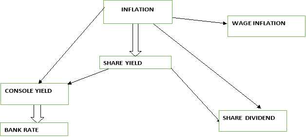Fig 3.1: Structure of Wilkie model Figure 2.1. The Cascade Structure of the Wilkie model. The parts of the Wilkie Model development in the UK included four fundamental variables, and these are:

Retail price index (Q)
Share dividends index (D)
Dividend yield (Y) on share price index (P)
Consols yield or long–term government interest rate (C).

Each of the variables are modeled within a cascade structure such that they are ordered from the top level to the lower levels. The values of the lower level variables depend on the lagged value of themselves and the values of the variables in the upper levels (Chao, 2007). Chao (2007) explains that the inflation rate, which is calculated from the change of retail price index, depends on its own lagged values and is placed on the top layer of the structure.

The forecast of this variable depends on its historical evidence. Chao (2007) describes the dividend yield as being in the second layer, and that its prediction is based on both the historical evidence and that of inflation rate; and finally, the third layer includes dividend and consols, whose forecast are based on the historical data, that of dividend yield, and that of inflation rate. The variables of the Wilkie (1986, 1995) were modeled under the following procedures:

Step one, the variables were modeled by the regression on the upper level variables.
Then, the models’ residuals were tested and constructed through the standard Box–Jenkins univariate time series modeling method.
Next, he tested other methods such as Vector Autoregressive (VAR) modeling of two correlated variables, and GARCH modeling for the variance of residuals.

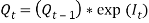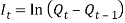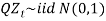
Formulae a. The Price Inflation Model. Inflation, as measured by the retail prices index (CPI), is modelled by a first order auto regressive (AR (l)) process. Wilkie’s AR (1) price inflation model is of the form: Where is the force of inflation over year (t-1) to (t) and it is given as: Hence: That is is a series of independent, identically distributed unit normal variates, (the assumption is that, they have zero mean and unit standard deviation). Where QMU, QA and QSD are parameters to be estimated. This model is described as that, each year the force of inflation is equal to its mean rate (QMU), plus a percentage of last year's deviation from the mean (QA), plus a random innovation which has zero mean and a standard deviation of QSD (Wilkie, 1986). The assumption is that, inflation, being the factor of economic uncertainty, depends only on past values of itself.

There is significant autocorrelation at lag 1, which provides statistical justification for inclusion of the variable, and no other economically plausible autocorrelation or partial autocorrelation is significant at 95% (Whitten &Thomas, 1995). The AR (1) model of the force of inflation is a statistically stationary series (i.e. in the long run the mean and variance are constant), of a b. Share Yields model Share yields are modelled as a function of the current inflation rate and the history of their past trends. The Wilkie’s AR (1) model of the share dividend yield is given as: That is, is a series of independent, identically distributed unit normal variates, (the assumption is that, they have zero mean and unit standard deviation). Where, YMU, YA, YW and YSD are parameters to be estimated.

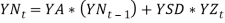
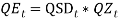
This model uses logarithmic transformed dividend yield, as the response variable. Wilkie (1995) described the model as that, at any date the logarithm of the dividend yield is equal to its mean value (ln YMU), plus a percentage of its deviation a year ago (YA) from the mean, plus an additional influence from inflation (YW) times the force of inflation in the previous year, plus a random innovation which has zero mean and a standard deviation of YSD. c. The Dividends model The model for share dividends, where is the value of a dividend index on ordinary shares at time t, is give as: Defining as the logarithm of the increase in the share dividends index from year to year , the Wilkie’s MA(1) dividend yield model can also be represented as: Where, . Hence, Wilkie (1985,1995) modeled for P(t), the value of a price index of ordinary shares at time t as: Or . That is, is a series of independent, identically distributed unit normal variates, (the assumption is that, they have zero mean and unit standard deviation). Where, DMU, DB, DW, DX, DSD, DY and DD are parameters to be estimated. Wilkie (195) described the model in words as: “in each year the change in the logarithm of the dividend index is equal to a function of current and past values of inflation, plus a mean real dividend growth (which is taken as zero), plus an influence from last year's dividend yield innovation, plus an influence from last year's dividend innovation, plus a random innovation which has zero mean and a standard deviation ( DSD).”

Long Term Interest Rate

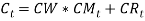
The long term interest rate model is for the Consols yield The model is based on , which is adjusted the long memory effect of inflation rate. The Wilkie’s AR(1) consols yield model is presented as: This part is an exponentially weighted average of current and past price inflation, standing the expected future inflation over the life of the bond. This is a zero-mean AR (1) process which is independent of price inflation, and controls the long-term real interest rate. That is, is a series of independent, identically distributed unit normal variates, (the assumption is that, they have zero mean and unit standard deviation). Where, CMU, CW, CA, CSD, and CD are parameters to be estimated.

The model is composed of two parts: an expected future inflation and a real yield (Sahin, et tal.). The portion representing the inflation part is modelled as a weighted moving average whiles the real part is modelled is an AR (1) with a contribution from the dividend yield. The parameter, CW = 1, which implies that, the model takes into account, the “Fisher effect”, in which the nominal yield on bonds reflects both expected inflation over the life of the bond and a ’real’ rate of interest Sahin, et tal.). Wilkie (1995) defines the logarithm of the real interest component as a linear autoregressive order one or three AR (1) or AR (3) but preferred the AR (1) model. e. Short Term Interest Rate (Bank Rate) Aside the fundamental parts of the Wilkie model, I consider one of the subsequent variables modelled by wilkie (1995).

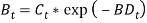
Wilkie used bank rate or bank base rate series to model short-term interest rates. Short-term interest rates are clearly connected with long-term ones. Wilkie’s approach was to model the difference between the logarithms of the difference of these series where is the value of bank rate at time t. That is, is a series of independent, identically distributed unit normal variates, (the assumption is that, they have zero mean and unit standard deviation). Where, BMU, BA, and BSD, are parameters to be estimated.

3.4.2 THE ARCH MODEL The Wilkie ARCH Model

The initial model developed by Wilkie (1986) assumed that the residuals of the inflation model were normally distributed. In 1995, he re-examined his own model and observed that the residuals were much fatter tailed than a normal distribution. In Statistics and Econometrics, one of the ways to model these fat tailed distributions is using an Autoregressive Conditional Heteroscedastic (ARCH) model (Engle, 1982).

In an Autoregressive Conditional Heteroschedastic (ARCH) model, the variance of the innovation term is modelled as a separate process (rather than assumed to be constant) (Wright, 2004). After the re-examination of the historical data, Wilkie (1995) proposed an ARCH model for the standard deviation of the inflation model. The ARCH model was seen to describe the data better than the original model by Huber (1997) and was suggested that, it should generally be used in applications of the model, unless the ARCH effect is not significant for those particular applications. In this ARCH model the varying value of the standard deviation, QSD(t), is made to depend on the previously observed value of the principal variable, I(tâˆ’1), which itself is modelled by an autoregressive series. The suggested model (with a slight alteration in the notation) was: That is, is a series of independent, identically distributed unit normal variates, (the assumption is that, they have zero mean and unit standard deviation). Where, QMU, QA QSA QSB, and QSC, are parameters to be estimated. This implies that the variation depends on how far away last year’s rate of inflation, , was from some middle level, QSC (similar to the mean, QMU), but with the deviation squared, so that extreme values of inflation in either direction would increase the variance (Sahin, 2010). Comparing the ARCH model to the initial autoregressive model showed that, the distribution of the force of price inflation) exhibits fatter tails and a greater concentration around the long-term mean value (Wright, 2004). The ARCH variation was incorporated in only the price inflation model.

Therefore, the remainder of the series follow the modelling as in the initial Wilkie model since Wilkie (1995) found no basses to re-model them as ARCH models. The ARCH model appears to give a better representation of inflation than the models assuming constant variance.

3.4.3 THE WHITTEN AND THOMAS MODEL

Whitten and Thomas model The main underpinning belief for this model is that, “the economy behaves differently in times of hyperinflation, than it does in times of normal inflation levels” Whitten & Thomas (1999).

This belief is non-linear in nature and hence could not have been modelled linearly. After vigorous exploration of several alternative, Whitten & Thomas (1999) adapted the Wilkie model (linear model) to incorporate their non-linearity assumption, rather than fundamentally changing the whole formulation. Whitten & Thomas (1999) did not model the heteroscedastic nature of the price inflation using the ARCH model as in Wilkie (1995) due to the challenges in estimating the model since and that it can give rise to troubling results from simulation. Whitten & Thoma (1999) employed the threshold modelling technique since threshold models are also capable of representing conditional variance, and moreover, exhibit short-term changes in mean. They proposed two regimes for each of the variables. The processes in each regime are similar to those defined by Wilkie (1986;1995).

Following the same cascade structure above, the formulae for the models are given below: The Price Inflation Model Inflation is assumed to be represented as a SETAR (self-exciting threshold autoregressive) model, with delay 1, and a threshold that differentiates between normal and high inflation. They fitted many different threshold models. Due to the paucity of data partitioned into the upper regime, it was difficult to postulate any sort of autocorrelation structure in the hyperinflation regime Whiten & Thomas (1999). The final suitable for threshold model for the price inflation is SETAR (2; 1, 0), thus: 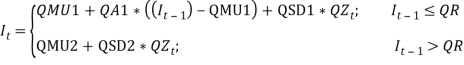That is is a series of independent, identically distributed unit normal variates, (the assumption is that, they have zero mean and unit standard deviation). Where QMU1, QA1, QSD1, QMU2, and QSD2 are parameters to be estimated. The model is described as that if the inflation in the previous year was below a certain threshold (QR), then the expected force of inflation () is equal to its mean (QMU1), plus a percentage of last year’s deviation from the mean (QA1) plus a random innovation which has zero mean and standard deviation QSD1. Conversely if the inflation in the previous year was above the threshold, then the expected force of inflation presently is equal to its mean (QMU2), plus a random innovation which has zero mean and standard deviation QSD2.

The model is able to control heteroscedasticity in a way because the expected variance of inflation when it is in its excited phase is greater than when it is in its quiescent phase Whitten & Thomas (1999). The dividend model Following Wilkie (1986, 1995), Whitten & Thomas (1999) also represented the share divided series as moving average of order one (MA (1)). Defining as in the Wilkie model as the logarithm of the increase in the share dividends index from year t-1 to t, this model is similar to the Wilkie model but with the introduction of a normal and a high inflation regimes. In economic sense, dividends do better in times of normal inflation, than in times of high inflation therefore, the model employs the condition that 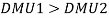The model for is of the form: Where, 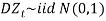That is is a series of independent, identically distributed unit normal variates, (the assumption is that, they have zero mean and unit standard deviation). Where Where, DMU1 DMU2, DB, DW, DX, DSD, DY and DD are parameters to be estimated. The share yield model Our share yield model is different to Wilkie.s lnY(t) in that we include a transfer effect from a+lnC(t) to YN(t). lnY(t) was re-estimated a TAR model, with extra parameters YY1 and YY2, to include this transfer, i.e. 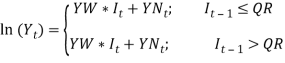where, 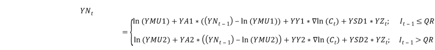That is, is a series of independent, identically distributed unit normal variates, (the assumption is that, they have zero mean and unit standard deviation). Where, YMU, YA, YW and YSD are parameters to be estimated. consol It is not easy to estimate the exponential smoothing parameter, CD, for each regime in C(t). There are problems when using a more sensitive smoothing parameter, in that {C(t) . CM(t)} > 0, i.e. we cannot allow a negative real interest rate. It seemed a necessary simplification to have the allowance for expected future inflation over the life of the bond (CM(t)), and hence the parameter CD, defined the same for each regime. It therefore follows that, like the Wilkie model, our model gives a unit gain between inflation and interest rates. 4.4.6 C(t) was then re-estimated as a TAR model, i.e. 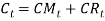short term interest rate BD(t) was re-estimated as a TAR model, i.e.